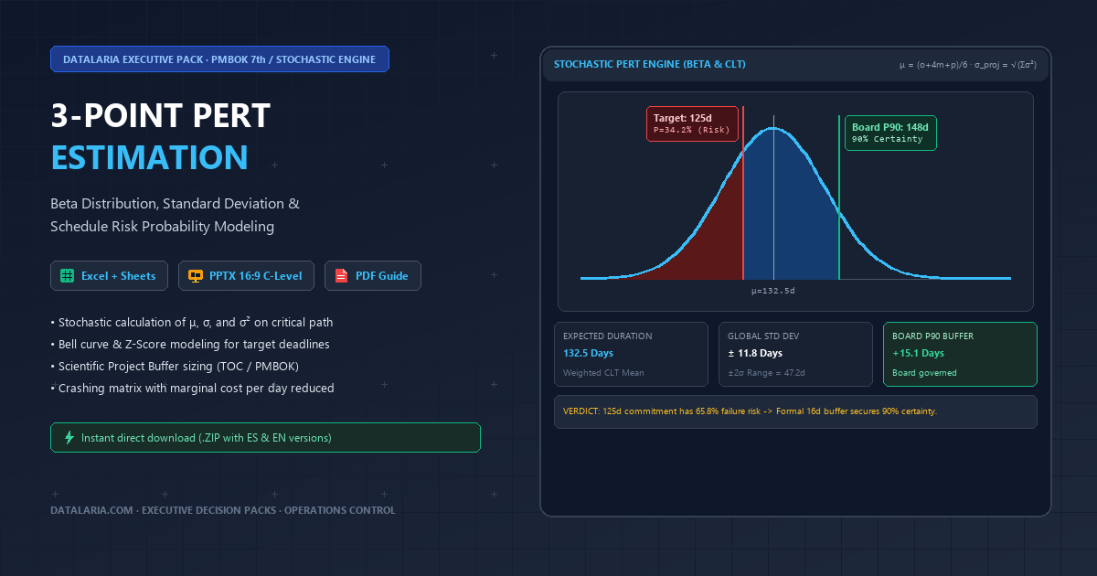
In executive committees, corporate boards of directors, and investment steering committees, Chief Executive Officers (CEOs), Chief Operating Officers (COOs), Chief Technology Officers (CTOs), and Project Management Office (PMO) leaders consistently face a recurring structural pathology known in operations research and Tier-1 strategy consulting as “the deterministic last-mile fallacy”:
An engineering, cloud architecture, or enterprise infrastructure team spends weeks decomposing project scope into a detailed Work Breakdown Structure (WBS). The final presentation culminates in an elegant linear Gantt chart where each activity is tagged with an absolute static duration: “Core clearing engine development: 18 days”, “Banking API integration: 14 days”, “User Acceptance Testing (UAT): 12 days”. By summing these deterministic line items across dependencies, the project sponsor solemnly announces to the Board: “Go-Live is firmly scheduled for October 15th”.
Yet, when the target date arrives, the project is invariably weeks or months behind schedule. Faced with executive frustration and commercial penalties, technical leads routinely attribute the slippage to “unprecedented external friction”, “unexpected vendor bottlenecks”, or “shifting requirements”.
The mathematical reality is far more objective: the initiative did not derail due to bad operational luck; it was statistically doomed before the first line of code was ever committed.
By demanding or accepting a single static date (a deterministic single-point estimate), corporate leadership falls victim to four well-documented operational traps:
- The Asymmetry of Engineering Risk: In complex software development and systems engineering, duration distributions are never symmetrical bell curves. While favorable breakthroughs rarely shave more than 15-20% off task durations, unanticipated technical friction (API breaking changes, key talent turnover, architectural defects) easily inflates timelines by two, three, or four times. Relying on a single modal value completely ignores the heavy right-tail of the distribution.
- Parkinson’s Law: Formulated by Cyril Northcote Parkinson in 1957, this law states that “work expands to fill the time available for its completion”. If an engineering team finishes core logic in 9 days for a 15-day allocated task, the remaining 6 days are almost never handed back to the critical path; they are consumed by secondary refactoring, cosmetic polish, or relaxed delivery pacing. Early gains are never accumulated across work packages.
- Student Syndrome & Invisible Buffer Dissipation: When engineers are pressured to commit to rigid dates, they informally embed hidden safety padding inside their estimates. However, because they know buffer exists, focused execution is postponed until the milestone is immediately looming. When the first genuine impediment emerges near delivery, the individual safety margin has already been consumed, transmitting 100% of the delay downstream into the critical path.
- The Joint Probability Trap of Critical Sequences: If a critical path comprises 15 sequential tasks each estimated at an unhedged 50% median probability of on-time completion, the joint mathematical probability of all tasks finishing on schedule independently is $(0.5)^{15} = 0.0000305$ (barely 0.003%). Committing to the direct sum of task medians is mathematically indistinguishable from guaranteeing operational failure.
To eliminate this structural vulnerability and establish a board-grade governance framework, the Project Management Institute (PMI) in the PMBOK Guide 7th Edition, Operations Research, and Theory of Constraints (TOC / Critical Chain) establish the Stochastic 3-Point PERT Estimation Engine.
In this executive guide, we examine the underlying mathematics of the Beta Distribution, Central Limit Theorem (CLT) variance aggregation, structured pre-mortem interview techniques to neutralize anchoring bias, Z-Score calculations for contractual deadlines, scientific Theory of Constraints buffer sizing (Project Buffers), and the executive boardroom defense protocol.
Executive Decision Pack: Stochastic 3-Point PERT Estimation
1. What Is Stochastic 3-Point PERT Estimation? Core Mechanics & Executive Goals
For any engineering lead, PMO manager, or executive encountering probabilistic schedule modeling for the first time, the PERT methodology (Program Evaluation and Review Technique) replaces the illusion of a single fixed Go-Live date with a bounded statistical range defined by three independent estimates per WBS work package:
- Optimistic Estimate ($o$): The minimum physically achievable duration if technical execution, external dependencies, and team availability align exceptionally well (roughly the $P_5$ percentile).
- Most Likely Estimate ($m$): The realistic modal duration under standard operating conditions, assuming neither heroic breakthroughs nor catastrophic blockers.
- Pessimistic Estimate ($p$): The worst-case duration under severe operational friction—breaking vendor APIs, specialist turnover, security audit remediation—excluding force majeure catastrophes (roughly the $P_{95}$ percentile).
From this $(o, m, p)$ triad, the engine computes an auditable Beta expected duration ($\mu = \frac{o + 4m + p}{6}$) and individual variance ($\sigma^2 = \left(\frac{p - o}{6}\right)^2$), aggregating them along the Critical Path via the Central Limit Theorem (CLT) to quantify true completion odds.
1.1 Four Strategic Objectives for Boardroom Governance
Adopting a Stochastic PERT framework over static Gantt planning serves four concrete executive governance goals:
- Replace deterministic promises with auditable probabilities ($P(T \le T_d)$): Enable leadership to see instantly whether a commercial milestone holds a $34\%$ or $90\%$ statistical chance of success before signing SLA-backed client contracts.
- Decouple engineering execution from contingency reserves: Consolidate hidden task-level padding into a transparent, PMO-governed Project Buffer (following Goldratt’s Theory of Constraints / Critical Chain), eliminating Parkinson’s Law and Student Syndrome.
- Optimize schedule acceleration capital (Crashing ROI): Identify precisely which Critical Path tasks yield the lowest marginal cost per day reduced (USD/day) when schedule compression is mandatory before Go-Live.
- Standardize executive risk appetite across initiatives: Establish explicit corporate confidence gates ($P_{80}$ for agile internal programs, $P_{90}$ for enterprise client go-lives, $P_{95}\text{–}P_{99}$ for mission-critical infrastructure).
1.2 Traditional Deterministic Scheduling vs. Stochastic 3-Point PERT
| Analytical Dimension | Deterministic Planning (Single-Point) | Stochastic 3-Point PERT (PMBOK 7th / CLT) |
|---|---|---|
| Estimation unit | A single static number (typically optimistic or modal $m$). | Triad $(o, m, p)$ explicitly capturing right-tail risk skewness. |
| Implied on-time probability | $\le 50\%$ per activity; approaches $0\%$ across $\ge 10$ sequential critical tasks. | Continuous cumulative curve $\Phi(Z)$ evaluated against any deadline $T_d$. |
| Uncertainty handling | Hidden local padding inside every task (wasted by Parkinson’s Law). | Quadratic variance aggregation $\sigma^2 = ((p-o)/6)^2$ feeding a governed Project Buffer. |
| Acceleration strategy | Unfocused executive pressure (“all-hands crunch & overtime”). | Ranked Crashing Matrix prioritized strictly by lowest marginal cost per day saved. |
| Boardroom auditability | Subjective and fragile when the first blocker hits. | Mathematically reproducible across Excel 365 and Google Sheets. |
1.3 Connecting PERT to Datalaria’s Strategic-Operational Funnel
Stochastic schedule estimation does not operate in a vacuum—it forms the timeline assurance layer inside Datalaria’s end-to-end Corporate Strategy, Investment Decision, and Operational Control architecture:
- Layer 1 · Corporate Strategy & Portfolio Selection (Suite 01): Before locking timelines, leadership validates strategic fit via the Quantitative SWOT & TOWS Matrix, macro volatility mapping with the Quantitative PESTEL Matrix, industry structure analysis using Weighted Porter’s 5 Forces, Dynamic BCG Portfolio Matrix, and McKinsey / GE 3x3 Matrix, synthesized in the Quantitative Corporate Strategy Framework.
- Layer 2 · Rational Decision-Making & Capital Prioritization (Suite 02): Candidate initiatives pass veto screening in the Quantitative DAR Matrix, rank by impact-to-effort via the RICE & ICE Prioritization Matrix, and prove capital viability in the Financial Business Case (NPV, IRR & Payback), integrated in the 3-Tier Rational Decision-Making Framework.
- Layer 3 · Operational Control & Execution Governance (Suite 03): Once approved, execution eliminates ownership bottlenecks via the Quantitative RACI & Workload Matrix, scores failure modes with the Quantitative Risk Matrix & Operational FMEA (RPN), and locks schedule certainty with this Stochastic 3-Point PERT engine before active delivery tracking (Earned Value Management / EVM) and inventory protection (Safety Stock & ROP).
2. The Stochastic Schedule Governance Lifecycle
Probabilistic schedule control is not an academic exercise; it represents a closed-loop engineering workflow connecting mathematical variance with corporate risk appetite:
Isolating modular, independent work packages
Mapping functional dependencies and predecessor links"] B["2. Structured 3-Point Elicitation Protocol
Bias-free calibration: Optimistic (o), Most Likely (m), Pessimistic (p)
Pre-Mortem questioning to capture 95th percentile worst-case"] C["3. Beta PERT Statistical Computation
Expected mean: μ = (o + 4m + p) / 6
Individual standard deviation: σ = (p - o) / 6
Individual variance: σ² = [ (p - o) / 6 ]²"] D["4. Critical Path Method (CPM) Isolation
Identifying the longest continuous sequence of dependent tasks
Separating critical activities from feeder paths with float"] E["5. Central Limit Theorem (CLT) Aggregation
Total expected project duration: Σμcrit
Quadratic aggregation of variances: σproj² = Σσcrit²
Global standard deviation: σproj = √(Σσcrit²)"] F{"6. Target Deadline Z-Score Audit
Z = (Td - μtotal) / σtotal
Cumulative success probability: P(T ≤ Td) = Φ(Z)
Is P ≥ 90% certainty?"} G["HIGH-RISK DEADLINE GAP (P < 90%)
Unviable commitment before Executive Board
Mandatory activation of stochastic adjustment levers"] H["7. Scientific Buffer Sizing & Crashing
TOC Root-Sum-Square (RSS) Project Buffer at P90 (1.282σ)
Crashing matrix: Selective reduction by lowest marginal cost ($/day)"] I["8. Board Decision Gateway
Formal delivery lock at P90 confidence threshold
PMO-governed contingency reserve sign-off & C-Level approval"] A --> B B --> C C --> D D --> E E --> F F -->|"No: Probability Deficit"| G G --> H H --> E F -->|"Yes: Board Threshold Met"| I style A fill:#F8FAFC,stroke:#64748B,stroke-width:1.5px,color:#0F172A style B fill:#EFF6FF,stroke:#3B82F6,stroke-width:1.5px,color:#1E3A8A style C fill:#0F172A,stroke:#2563EB,stroke-width:2px,color:#FFFFFF style D fill:#EFF6FF,stroke:#2563EB,stroke-width:1.5px,color:#1E3A8A style E fill:#0F172A,stroke:#0284C7,stroke-width:2px,color:#FFFFFF style F fill:#FEF3C7,stroke:#F59E0B,stroke-width:2px,color:#92400E style G fill:#FEE2E2,stroke:#DC2626,stroke-width:2px,color:#991B1B style H fill:#EFF6FF,stroke:#3B82F6,stroke-width:1.5px,color:#1E3A8A style I fill:#D1FAE5,stroke:#10B981,stroke-width:2px,color:#065F46
🔍 Haz clic en el diagrama para ampliarlo a pantalla completa
This lifecycle ensures that the project timeline presented to the Executive Committee is an actuarially sound model rather than an optimistic executive wish list.
3. Mathematical Foundations & Quantitative Mechanics
To build an auditable model computable in executive spreadsheets, schedule uncertainty across every work package must be modeled as a continuous random variable.
3.1 The Beta Distribution as a Duration Engine
Engineered in 1959 by the US Navy Special Projects Office and Booz Allen Hamilton (Malcolm et al., 1959) for the submarine-launched Polaris ballistic missile program, PERT (Program Evaluation and Review Technique) replaced single-point estimates with a continuous Beta Distribution bounded within the interval $[o, p]$.
The Beta distribution is exceptionally suited for engineering project modeling:
- Finite Boundaries: It defines an absolute minimum physical duration ($o$) and a realistic worst-case duration ($p$).
- Flexible Skewness: It accommodates an asymmetric mode ($m$) situated closer to the optimistic bound, reflecting the natural real-world reality where technical setbacks outnumber early breakthroughs.
To enable operational computation without requiring complex numerical calculus in day-to-day project management, PERT established the canonical polynomial approximations, assuming that the entire range spans approximately six standard deviations ($6\sigma = p - o$):
A. Expected PERT Beta Duration ($\mu_i$)
$$\mu_i = \frac{o + 4m + p}{6}$$This weighted average assigns a $4/6 \approx 66.7\%$ weight to the most likely mode ($m$), and $1/6 \approx 16.7\%$ to each extreme tail ($o$ and $p$). Note that under positive right-skewness ($p - m > m - o$), the expected mean $\mu_i$ is strictly greater than the mode $m$.
B. Triangular Mean Comparison ($\mu_{tri}$)
$$\mu_{tri} = \frac{o + m + p}{3}$$Triangular distributions calculate an unweighted average. In highly volatile environments, this approach overweights extreme outliers, creating unnecessary distortion compared to the balanced Beta formulation.
C. Individual Standard Deviation ($\sigma_i$)
$$\sigma_i = \frac{p - o}{6}$$The standard deviation quantifies the intrinsic volatility of the deliverable. A well-defined work package ($o=9, p=12$) yields $\sigma = 0.5$ days (high certainty), whereas an exploratory research task ($o=5, p=29$) yields $\sigma = 4.0$ days (high uncertainty).
D. Individual Variance ($\sigma_i^2$)
$$\sigma_i^2 = \left(\frac{p - o}{6}\right)^2$$Variance measures quadratic dispersion and serves as the essential building block for aggregate critical path analysis.
E. Skewness Ratio
$$\text{Skewness} = \frac{(p - m) - (m - o)}{p - o} = \frac{o + p - 2m}{p - o}$$- $\text{Skewness} > 0$ (Right-Skewed): Extended tail of potential technical slippage. Represents 85-90% of real-world software and engineering initiatives.
- $\text{Skewness} = 0$ (Symmetrical): Mode is perfectly centered ($m = (o + p)/2$).
- $\text{Skewness} < 0$ (Left-Skewed): Rare scenarios with fixed hard deadlines and high automation upside.
3.2 Critical Path Aggregation: The Central Limit Theorem (CLT)
The fatal flaw of deterministic planning is the linear addition of static task numbers. In stochastic project management, network aggregation is governed by the Central Limit Theorem (CLT).
The CLT states:
Given a sequence of independent random variables $X_1, X_2, \dots, X_n$, each with finite mean $\mu_i$ and finite variance $\sigma_i^2$, the distribution of their sum $S_n = \sum_{i=1}^n X_i$ asymptotically converges toward a Gaussian Normal Distribution as $n$ increases, regardless of the underlying distribution shapes of the individual components.
Applied to project networks:
- The Critical Path activities dictate overall project completion time.
- Even if individual tasks follow skewed Beta distributions, total project duration converges to a Normal Distribution:
Global project parameters are calculated as follows:
1. Total Expected Project Duration ($\mu_{total}$)
$$\mu_{total} = \sum_{i \in \text{Critical}} \mu_i = \sum_{i \in \text{Critical}} \frac{o_i + 4m_i + p_i}{6}$$2. Combined Project Variance ($\sigma_{total}^2$)
Under the assumption of task independence, variances are summed quadratically, never standard deviations linearly:
$$\sigma_{total}^2 = \sum_{i \in \text{Critical}} \sigma_i^2 = \sum_{i \in \text{Critical}} \left(\frac{p_i - o_i}{6}\right)^2$$3. Global Project Standard Deviation ($\sigma_{total}$)
$$\sigma_{total} = \sqrt{\sigma_{total}^2} = \sqrt{\sum_{i \in \text{Critical}} \left(\frac{p_i - o_i}{6}\right)^2}$$The Mathematical Power of CLT Aggregation:
$$\sum \sigma_i = 1 + 1 + \dots + 1 = 9 \text{ days}$$
Consider 9 independent critical tasks, each with an uncertainty span of 6 days ($p - o = 6$), meaning each task has $\sigma_i = 1$ day.
If an evaluator adds standard deviations linearly (a naive worst-case approach), the apparent project dispersion would be:
$$\sigma_{total} = \sqrt{1^2 + 1^2 + \dots + 1^2} = \sqrt{9} = \mathbf{3 \text{ days}}$$
However, probability theory proves that individual fluctuations partially offset each other (some tasks finish slightly early, others slightly late). The true standard deviation of the project according to the CLT is:
The stochastic model demonstrates that aggregate uncertainty is three times smaller than the sum of individual worst-case fears! This prevents leadership from unnecessarily inflating project budgets and losing commercial competitiveness.
3.3 Z-Score Calculation & Success Probability for Target Deadlines
With $\mu_{total}$ and $\sigma_{total}$ established, the model answers the ultimate executive question:
“What is the exact probability of delivering the project on or before committed deadline $T_d$?”
We standardize the normal distribution by calculating the Z-Score:
$$Z = \frac{T_d - \mu_{total}}{\sigma_{total}}$$Here, $Z$ represents the number of standard deviations separating the deadline $T_d$ from the project mean $\mu_{total}$. Cumulative success probability is then evaluated via the Cumulative Normal Distribution Function ($\Phi$):
$$P(T \le T_d) = \Phi(Z) = \frac{1}{\sqrt{2\pi}} \int_{-\infty}^{Z} e^{-\frac{u^2}{2}} \, du$$In Microsoft Excel and Google Sheets, this is computed instantaneously using:
=NORM.DIST(T_d, mu_total, sigma_total, TRUE) or =NORMSDIST(Z).
Executive Z-Score Decision Framework
| Target Confidence $P(T \le T_d)$ | Standard Z-Score | Time Expression ($T_d$) | Executive Diagnosis & Risk Profile |
|---|---|---|---|
| 50.0% | $Z = 0.000$ | $\mu$ | Coin toss. 50% delay risk. Unacceptable for Board commitments. |
| 60.0% | $Z = +0.253$ | $\mu + 0.25\sigma$ | High Risk. Severe exposure to contractual penalties and stakeholder friction. |
| 70.0% | $Z = +0.524$ | $\mu + 0.52\sigma$ | Aggressive. Only acceptable for internal non-critical R&D iterations. |
| 75.0% | $Z = +0.674$ | $\mu + 0.67\sigma$ | Minimum Agile Baseline. Requires bi-weekly burn-rate telemetry. |
| 80.0% | $Z = +0.842$ | $\mu + 0.84\sigma$ | PMBOK Standard. Balanced alignment between buffer investment and certainty. |
| 85.0% | $Z = +1.036$ | $\mu + 1.04\sigma$ | Prudent. Low disruption risk for commercial client deliveries. |
| 90.0% | $Z = +1.282$ | $\mu + 1.28\sigma$ | ⭐ RECOMMENDED BOARDROOM C-LEVEL STANDARD. |
| 95.0% | $Z = +1.645$ | $\mu + 1.65\sigma$ | Mission Critical. Mandatory in core banking, cloud migrations, and medical tech. |
| 99.0% | $Z = +2.326$ | $\mu + 2.33\sigma$ | Zero Tolerance. Aerospace, defense, and life-support control software. |
4. Bias-Free 3-Point Elicitation Protocol
A stochastic model is only as sound as the inputs powering it. Behavioral economics (Kahneman & Tversky, 1979) demonstrates that when technical leads are casually asked for estimates, cognitive biases inevitably corrupt their inputs:
- Anchoring Bias: If a commercial sponsor states “we must launch by Q3”, technical leads unconsciously anchor their estimates around that date.
- Social Desirability Bias: Engineering managers fear being perceived as obstructionist or slow, leading them to compress estimates to please senior hierarchy.
To eliminate cognitive distortion, PMO teams must enforce a 4-step structured elicitation interview protocol:
Step 1: Eliciting the Most Likely Estimate ($m$)
- Guiding Prompt: “Assuming nominal staffing, normal operating cadence, and no catastrophic friction, what is the most frequent and realistic duration required to complete this deliverable?”
- Governance Rule: Never display the overall project deadline during this step to prevent cross-anchoring.
Step 2: Isolating the Pessimistic Scenario ($p$) via Pre-Mortem
- Guiding Prompt: “Imagine we travel 6 months into the future and this specific work package has experienced severe friction: the third-party API introduced breaking changes, the vendor had key personnel turnover, and data sanitization required major rework. Excluding extreme force majeure acts of God, what is the realistic worst-case duration?”
- Calibration Rule: Assign $p$ to the 95th percentile (a duration exceeded only 1 in 20 times under real-world conditions).
Step 3: Isolating the Optimistic Scenario ($o$)
- Guiding Prompt: “If contracts clear in 24 hours, zero tech debt is uncovered, vendor dependencies deliver on day one, and the engineering squad works in uninterrupted flow, what is the absolute physical minimum duration to ship this deliverable with full quality?”
- Calibration Rule: Assign $o$ to the 5th percentile (achievable only 1 in 20 times under ideal conditions).
Step 4: Skewness Ratio Verification
- If an engineer submits perfectly symmetrical estimates ($o=10$, $m=15$, $p=20$), the PMO must actively challenge the estimate. Real-world engineering tasks are consistently right-skewed ($(p - m) > (m - o)$). Perfect symmetry is almost always indicative of superficial subtraction and addition (e.g., $\pm 5$ days) rather than rigorous technical analysis.
5. Scientific Buffer Sizing & Schedule Crashing
One of the most transformative insights of the Theory of Constraints (TOC / Critical Chain), championed by Eliyahu Goldratt, is to strip individual tasks of hidden safety padding and consolidate protection into a transparent, centralized Project Buffer governed formally by the PMO.
5.1 Project Buffer Sizing Methodologies
Two quantitative approaches exist for sizing executive contingency buffers:
Method 1: Traditional Goldratt 50% Cut
$$\text{PB}_{50\%} = 0.5 \times \sum_{i \in \text{Critical}} (p_i - m_i)$$This heuristic takes half of the accumulated pessimistic uncertainty. While vastly superior to zero buffer, it assumes linear uncertainty accumulation, which often inflates project schedules excessively on large critical paths.
Method 2: Scientific Root-Sum-Square (RSS / CLT) Method
Grounded in the Central Limit Theorem, this method sizes the project buffer as a direct multiple of combined standard deviation:
$$\text{PB}_{RSS} = K \times \sigma_{total} = K \times \sqrt{\sum_{i \in \text{Critical}} \sigma_i^2}$$Where $K$ represents the target confidence coefficient approved by the Board:
- 80% Certainty: $K = 0.842 \implies \text{PB} = 0.842 \times \sigma_{total}$
- 90% Certainty (Board Standard): $K = 1.282 \implies \text{PB} = 1.282 \times \sigma_{total}$
- 95% Certainty (Mission Critical): $K = 1.645 \implies \text{PB} = 1.645 \times \sigma_{total}$
5.2 Critical Path Crashing: Marginal Cost per Day Reduced
When competitive pressures require compressing the schedule below the expected duration $\mu_{total}$, arbitrary overtime leads to burnout and ballooning costs.
The formal Schedule Crashing technique requires calculating the Marginal Cost Slope per Day Reduced ($S_i$) for every critical path deliverable:
$$S_i = \frac{\text{Crash Cost} - \text{Normal Cost}}{\text{Normal Duration} - \text{Crash Duration}} \quad [\$/\text{day}]$$Crashing Governance Rules
- Crash Critical Path Tasks Exclusively: Allocating capital to accelerate non-critical tasks does not shorten total project duration by a single day; it purely wastes capital.
- Prioritize by Lowest Cost Slope ($S_i$): Rank critical deliverables from lowest to highest marginal cost per day reduced. Crash the deliverable with the lowest $S_i$ until its compression limit is reached, then proceed to the next lowest.
- Monitor Near-Critical Paths: As the primary critical path is compressed, secondary parallel paths may become critical, altering global variance dynamics.
6. Enterprise Case Study: Core Cloud Transformation
To demonstrate boardroom impact, let us examine an enterprise financial institution overhauling its core transactional clearing engine:
6.1 Project Baseline Parameters
- Scope: 25 WBS work packages (cloud architecture, core ledger, banking gateways, SAP integration, Kafka streaming, PCI-DSS compliance, and staging cutover).
- Critical Path: 15 sequential tasks identified via CPM.
- Demanded Target Date: 125 business days (a fixed 6-calendar-month contractual milestone).
6.2 The Datalaria Stochastic Audit
Applying 3-point Beta estimation and Central Limit Theorem variance aggregation revealed the following metrics:
- Sum of Modal Estimates ($\sum m_{crit}$): 124.0 business days.
- Expected PERT Beta Duration ($\mu_{total} = \sum \mu_{crit}$): 132.5 business days.
- Combined Project Variance ($\sigma_{total}^2 = \sum \sigma_{crit}^2$): 139.24 days².
- Global Standard Deviation ($\sigma_{total} = \sqrt{139.24}$): 11.80 business days.
- 95.4% Confidence Interval ($\mu \pm 2\sigma$): [108.9 to 156.1 days].
6.3 Diagnostic Audit of the 125-Day Deadline
We compute the Z-Score and success probability for the mandated 125-day deadline:
$$Z = \frac{125.0 - 132.5}{11.80} = \frac{-7.5}{11.80} = \mathbf{-0.636}$$$$P(T \le 125) = \Phi(-0.636) = \mathbf{34.2\% \text{ Probability of Success}}$$The Boardroom Verdict:
The 125-day target demanded by executive sponsors had a 65.8% probability of public failure. Promising this deadline without contingency protection represented technical governance negligence.
6.4 Board Decision Gateway Execution
The leadership team presented the Bell Curve and sensitivity rankings using the official C-Level presentation format:
- Adopting the P90 Target Date (90% Certainty): $$T_{90} = \mu + 1.282 \times \sigma = 132.5 + 1.282 \times 11.80 = \mathbf{147.6 \text{ days}} \approx 148 \text{ business days}$$ The Board formally approved locking the contractual commitment at 148 days, establishing an official Project Buffer of 15.1 business days.
- Selective Crashing Reserve:
Three critical tasks were pre-selected for targeted acceleration:- User Acceptance Testing (UAT): $800/day (max 5 days saved for $4,000).
- Banking Gateway Integration: $950/day (max 4 days saved for $3,800).
- Core Ledger Reconciliation: $1,100/day (max 4 days saved for $4,400).
The Board pre-allocated a $12,200 contingency reserve triggered only if buffer penetration breached the Amber threshold.
- Operational Outcome:
The project encountered two unexpected banking regulatory certification delays (an 8-day slippage). Because the 15.1-day buffer was formally in place, the project went live on Day 142 with zero crisis firefighting, finishing 6 days ahead of the P90 Board commitment.
7. Boardroom Defense Protocol: Executive FAQ
When defending a stochastic schedule before the Board of Directors or Steering Committee, PMOs must address incisive executive inquiries with mathematical authority:
FAQ 1: “Why can’t we simply commit to the Most Likely ($m$) date provided by engineering leads?”
Executive Response: Committing to the mode ($m$) assumes a symmetrical world where upside gains perfectly match downside delays. Due to inherent engineering risk asymmetry, the mode typically corresponds to a percentile below 40%. Committing to $m$ is mathematically equivalent to accepting a 60% probability of public project failure. Fiduciary duty requires executive leadership to anchor corporate commitments at a minimum 85-90% certainty threshold.
FAQ 2: “Why can’t we just add up all the worst-case ($p$) estimates to be completely safe?”
Executive Response: Linearly adding all pessimistic estimates assumes that every independent risk materializes simultaneously at maximum severity. The joint probability of 15 independent tasks hitting their 95th percentile concurrently is $(0.05)^{15} \approx 3 \times 10^{-20}$—astronomically lower than the odds of a meteor strike. Central Limit Theorem proves that aggregate uncertainty grows with the square root of variances ($\sqrt{\sum \sigma^2}$), not line-item addition. Padding the project linearly would make our commercial proposal uncompetitive in the market.
FAQ 3: “What certainty threshold (80%, 90%, or 95%) should the Board mandate?”
Executive Response: This decision depends on the Cost of Delay and commercial penalty structures:
- Internal Agile Projects (P75 - P80): Moderate delay impact is manageable internally; maintaining lean delivery pressure is healthy.
- Enterprise Programs & Client Go-Lives (P90): Tier-1 international governance mandates P90 ($Z = 1.282$) to align marketing spend, inventory procurement, and client onboarding.
- Mission-Critical Systems (P95 - P99): Core banking engines, medical tech, and aerospace systems where a release delay or defect triggers existential financial penalties.
8. The Executive Decision Pack: Production-Ready Schedule Infrastructure
For operations directors, PMO leaders, management consultants, and executives who need to implement this analytical standard immediately without investing weeks in statistical model validation, Datalaria provides the official Executive Decision Pack:
Stochastic 3-Point PERT Estimation
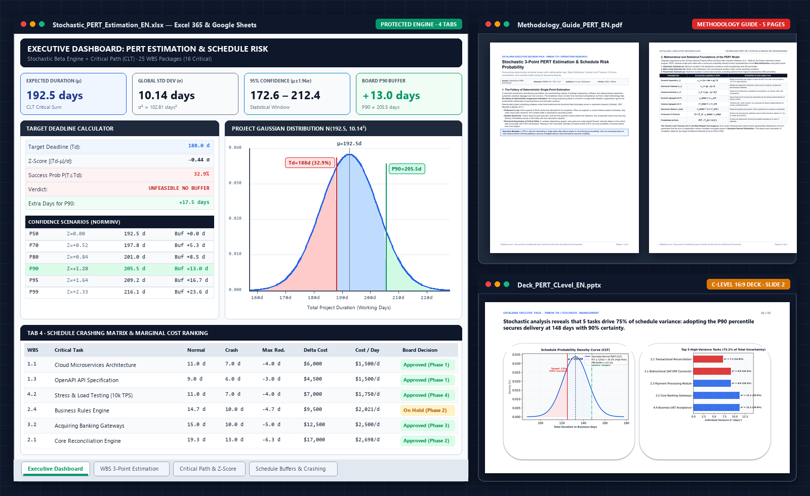 🔍 Actual preview of deliverables included: Stochastic Excel (.xlsx) engine with CLT Dashboard, Z-Score Deadline Calculator, Bell Curve and Crashing Matrix, Official Methodology Guide (.pdf), and C-Level 16:9 Board Deck (.pptx). (Click to enlarge)
- Probabilistic scheduling: Expected Duration, Variance, and Standard Deviation
- Commitment date probability engine (Beta Distribution & CLT)
- 16:9 C-Level Deck with Probability Density Bell Curve
- 5-page methodology guide with canonical PMBOK statistical formulas
- Instant direct download (.ZIP with bilingual ES & EN editions)
The Excel workbook features 100% editable input cells (white background) and statistical formulas protected under password provided in the instructions (ECMA-376 OpenXML standard). It includes the widescreen 16:9 PowerPoint deck structured under the Minto Pyramid and the 5-page editorial PDF methodology guide.
The master ZIP package contains fully localized and audited editions in both Spanish and English, Google Sheets import guides, and complete operational documentation.
9. Authoritative Canonical References
-
Project Management Institute (PMI) (2021). A Guide to the Project Management Body of Knowledge (PMBOK Guide) – 7th Edition: Schedule & Measurement Performance Domains. Project Management Institute, Newtown Square, PA.
The global reference standard formalizing 3-point estimation and quantitative schedule management. ISBN:978-1628256642. -
Malcolm, D. G., Roseboom, J. H., Clark, C. E., & Fazar, W. (1959). Application of a Technique for Research and Development Program Evaluation (PERT). Operations Research, Vol. 7, No. 5, pp. 646–669.
The seminal paper introducing the 3-point Beta distribution and critical path variance aggregation in the Polaris missile project. DOI:10.1287/opre.7.5.646. -
Goldratt, Eliyahu M. (1997). Critical Chain. The North River Press, Great Barrington, MA.
The foundational work proving Parkinson’s Law and Student Syndrome in project governance, introducing scientific Project Buffers. ISBN:978-0884271536. -
Meredith, Jack R., & Mantel, Samuel J. (2011). Project Management: A Managerial Approach (8th Edition). John Wiley & Sons, Hoboken, NJ.
Comprehensive academic treatise on probabilistic network scheduling (CPM/PERT) and stochastic uncertainty. ISBN:978-0470533024. -
Kerzner, Harold (2017). Project Management: A Systems Approach to Planning, Scheduling, and Controlling (12th Edition). John Wiley & Sons, Hoboken, NJ.
Authoritative reference on schedule crashing, earned value integration, and corporate project governance. ISBN:978-1119165354. -
Minto, Barbara (2009). The Pyramid Principle: Logic in Writing and Thinking. Financial Times / Prentice Hall, London.
The gold standard methodology developed at McKinsey & Company for structuring executive boardroom presentations and action-oriented governance gateways. ISBN:978-0273710516.